Top 21 r quantregforest tuyệt nhất 2022

Tác giả: khủng long www.rdocumentation.org

Ngày đăng khủng long : 17/5/2021

Xếp hạng khủng long : khủng long 3 ⭐ ( 92337 lượt đánh giá khủng long )

Xếp hạng khủng long cao nhất: 5 ⭐

Xếp hạng khủng long thấp nhất: 2 ⭐

Tóm tắt: khủng long Bài viết về quantregForest function – RDocumentation. Đang cập nhật…

Khớp với kết quả khủng long tìm kiếm: quantregForest (version 1.3-7) quantregForest: Quantile Regression Forests Description Quantile Regression Forests infer conditional quantile functions from data Usage quantregForest (x,y, nthreads=1, keep.inbag=FALSE, …) Arguments x A matrix or data.frame containing the predictor variables. y The response variable. nthreads…

Tác giả: khủng long cran.r-project.org

Ngày đăng khủng long : 22/8/2021

Xếp hạng khủng long : khủng long 5 ⭐ ( 4869 lượt đánh giá khủng long )

Xếp hạng khủng long cao nhất: 5 ⭐

Xếp hạng khủng long thấp nhất: 5 ⭐

Tóm tắt: khủng long Bài viết về CRAN – Package quantregForest. Đang cập nhật…

Khớp với kết quả khủng long tìm kiếm: quantregForest: Quantile Regression Forests Quantile Regression Forests is a tree-based ensemble method for estimation of conditional quantiles. It is particularly well suited for high-dimensional data. Predictor variables of mixed classes can be handled. The package is dependent on the package ‘randomForest’, written by Andy Liaw….

Tác giả: khủng long github.com

Ngày đăng khủng long : 3/1/2021

Xếp hạng khủng long : khủng long 3 ⭐ ( 49975 lượt đánh giá khủng long )

Xếp hạng khủng long cao nhất: 5 ⭐

Xếp hạng khủng long thấp nhất: 3 ⭐

Tóm tắt: khủng long R package – Quantile Regression Forests, a tree-based ensemble method for estimation of conditional quantiles (Meinshausen, 2006). – GitHub – lorismichel/quantregForest: R package – Quantile Regres…

Khớp với kết quả khủng long tìm kiếm: 2017-12-19 · Quantile Regression Forests is a tree-based ensemble method for estimation of conditional quantiles (Meinshausen, 2006). It is particularly well suited for high-dimensional data. Predictor variables of mixed classes can be handled. The package is dependent on the package ‘randomForest’, written by Andy Liaw. Installation…

Tác giả: khủng long www.rdocumentation.org

Ngày đăng khủng long : 2/3/2021

Xếp hạng khủng long : khủng long 2 ⭐ ( 76178 lượt đánh giá khủng long )

Xếp hạng khủng long cao nhất: 5 ⭐

Xếp hạng khủng long thấp nhất: 1 ⭐

Tóm tắt: khủng long Bài viết về predict.quantregForest function – RDocumentation. Đang cập nhật…

Khớp với kết quả khủng long tìm kiếm: An object of class quantregForest newdata A data frame or matrix containing new data. If left at default NULL, the out-of-bag predictions (OOB) are returned, for which the option keep.inbag has to be set to TRUE at the time of fitting the object. what Can be a vector of quantiles or a function….

Tác giả: khủng long rdrr.io

Ngày đăng khủng long : 10/3/2021

Xếp hạng khủng long : khủng long 2 ⭐ ( 56547 lượt đánh giá khủng long )

Xếp hạng khủng long cao nhất: 5 ⭐

Xếp hạng khủng long thấp nhất: 3 ⭐

Tóm tắt: khủng long Quantile Regression Forests infer conditional quantile functions from
data

Khớp với kết quả khủng long tìm kiếm: …

Tác giả: khủng long stackoverflow.com

Ngày đăng khủng long : 14/4/2021

Xếp hạng khủng long : khủng long 4 ⭐ ( 57695 lượt đánh giá khủng long )

Xếp hạng khủng long cao nhất: 5 ⭐

Xếp hạng khủng long thấp nhất: 1 ⭐

Tóm tắt: khủng long I am trying to use the quantregForest() function from the quantregForest package (which is built on the randomForest package.)
I tried to train the model using:
qrf_model <- quantregForest(x=…

Khớp với kết quả khủng long tìm kiếm: 2016-02-13 · I am trying to use the quantregForest() function from the quantregForest package (which is built on the randomForest package.) I tried to train the model using: qrf_model <- quantregForest(x=……

Tác giả: khủng long mran.microsoft.com

Ngày đăng khủng long : 2/6/2021

Xếp hạng khủng long : khủng long 3 ⭐ ( 90158 lượt đánh giá khủng long )

Xếp hạng khủng long cao nhất: 5 ⭐

Xếp hạng khủng long thấp nhất: 5 ⭐

Tóm tắt: khủng long Bài viết về Quantile Regression Forests – An R-Vignette. Đang cập nhật…

Khớp với kết quả khủng long tìm kiếm: 2016-04-11 · A method to plot data for class quantregForest is also made available in the package. With the command plot the 90 % prediction interval for out-of-bag prediction is plotted. The input object has to be of class quantregForest, see Figure 1 for the Ozone dataset. The red dots mark the observations which lie…

Tác giả: khủng long www.r-bloggers.com

Ngày đăng khủng long : 10/7/2021

Xếp hạng khủng long : khủng long 2 ⭐ ( 83656 lượt đánh giá khủng long )

Xếp hạng khủng long cao nhất: 5 ⭐

Xếp hạng khủng long thấp nhất: 5 ⭐

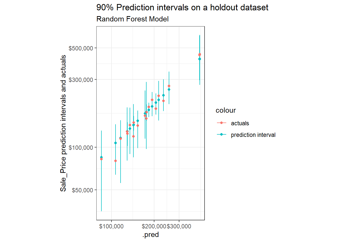
Tóm tắt: khủng long Quantile Regression Example Quantile Regression Forest Review Performance Coverage Interval Width Closing Notes Appendix Residual Plots Other Charts In this post I will build prediction intervals using quantile regression, more specifically, quantile regression forests. This is my third post on prediction intervals. Prior posts: Understanding Prediction Intervals (Part 1) Simulating Prediction Intervals (Part 2) This post should be read as a continuation on Part 11. I do not reintroduce terms, figures, examples, etc. that are initially described in that post2. My primary purpose here is to encode an example with the tidymodels suite of packages of building quantile regression forests for prediction intervals and to briefly review interval quality. Quantile Regression Rather than make a prediction for the mean and then add a measure of variance to produce a prediction interval (as described in Part 1, A Few Things to Know About Prediction Intervals), quantile regression predicts the intervals directly. In quantile regression, predictions don’t correspond with the arithmetic mean but instead with a specified quantile3. To create a 90% prediction interval, you just make predictions at the 5th and 95th percentiles – together the two predictions constitute a prediction interval. The chief advantages over the parametric method described in Part 1, Understanding Prediction Intervals are that quantile regression has… fewer and less stringent model assumptions. well established approaches for fitting more sophisticated model types than linear regression, e.g. using ensembles of trees. Advantages over the approach I describe in Simulating Prediction Intervals are… computation costs do not get out of control with more sophisticated model types4. can more easily handle heteroskedasticity of errors5. This advantage and others are described in Dan Saatrup Nielsen’s post on Quantile regression. I also recommend Dan’s post on Quantile regression forests for a description of how tree-based methods generate predictions for quantiles (which it turns out is rather intuitive). For these reasons, quantile regression is often a highly practical choice for many modeling scenarios that require prediction intervals. Example The {parsnip} package does not yet have a parsnip::linear_reg() method that supports linear quantile regression6 (see tidymodels/parsnip#465). Hence I took this as an opportunity to set-up an example for a random forest model using the {ranger} package as the engine in my workflow7. When comparing the quality of prediction intervals in this post against those from Part 1 or Part 2 we will not be able to untangle whether differences are due to the difference in model type (linear versus random forest) or the difference in interval estimation technique (parametric or simulated versus quantile regression). A more apples-to-apples comparison would have been to abandon the {parsnip} framework and gone through an example using the {quantreg} package for quantile regression… maybe in a future post. Quantile Regression Forest Starting libraries and data will be the same as in Part 1, Providing More Than Point Estimates. The code below is sourced and printed from that post’s .Rmd file. Load packages: library(tidyverse) library(tidymodels) library(AmesHousing) library(gt) # function copied from here: # https://github.com/rstudio/gt/issues/613#issuecomment-772072490 # (simpler solution should be implemented in future versions of {gt}) fmt_if_number % fit(ames_train) Review Tidymodels does not yet have a predict() method for extracting quantiles (see issue tidymodels/parsnip#119). Hence in the code below I first extract the {ranger} fit object and then use this to make predictions for the quantiles. preds_bind % bake(data_fit), type = “quantiles”, quantiles = c(lower, upper, 0.50) ) %>% with(predictions) %>% as_tibble() %>% set_names(paste0(“.pred”, c(“_lower”, “_upper”, “”))) %>% mutate(across(contains(“.pred”), ~10^.x)) %>% bind_cols(data_fit) %>% select(contains(“.pred”), Sale_Price, Lot_Area, Neighborhood, Years_Old, Gr_Liv_Area, Overall_Qual, Total_Bsmt_SF, Garage_Area) } rf_preds_test % mutate(pred_interval = ggplot2::cut_number(Sale_Price, 10)) %>% group_by(pred_interval) %>% sample_n(2) %>% ggplot(aes(x = .pred))+ geom_point(aes(y = .pred, color = “prediction interval”))+ geom_errorbar(aes(ymin = .pred_lower, ymax = .pred_upper, color = “prediction interval”))+ geom_point(aes(y = Sale_Price, color = “actuals”))+ scale_x_log10(labels = scales::dollar)+ scale_y_log10(labels = scales::dollar)+ labs(title = “90% Prediction intervals on a holdout dataset”, subtitle = “Random Forest Model”, y = “Sale_Price prediction intervals and actuals”)+ theme_bw()+ coord_fixed() If we compare these against similar samples when using the analytic and simulation based approaches for linear regression models, we find that the width of the intervals vary substantially more when built using quantile regression forests. Performance Overall model performance on a holdout dataset is similar (maybe slightly better) for an (untuned) Quantile Regression Forest9 compared to the linear model (MAPE on holdout dataset of 11% vs. 11.8% with linear model)10. As discussed in Part 1, Cautions With Overfitting, we can compare performance on train and holdout datasets to provide an indicator of overfitting: rf_preds_train % mutate(dataset = c(“training”, “holdout”)) %>% gt::gt() %>% gt::fmt_number(“.estimate”, decimals = 1) .metric .estimator .estimate dataset mape standard 4.7 training mape standard 11.0 holdout We see a substantial discrepancy in performance11. This puts the validity of the expected coverage of our prediction intervals in question12… Coverage Let’s check our coverage rates on a holdout dataset: coverage % mutate(covered = ifelse(Sale_Price >= .pred_lower & Sale_Price % group_by(…) %>% summarise(n = n(), n_covered = sum( covered ), stderror = sd(covered) / sqrt(n), coverage_prop = n_covered / n) } rf_preds_test %>% coverage() %>% mutate(across(c(coverage_prop, stderror), ~.x * 100)) %>% gt::gt() %>% gt::fmt_number(“stderror”, decimals = 2) %>% gt::fmt_number(“coverage_prop”, decimals = 1) n n_covered stderror coverage_prop 731 706 0.67 96.6 Surprisingly, we see a coverage probability for our prediction intervals of >96%13 on our holdout dataset14 – greater than our expected coverage of 90%. This suggests our prediction intervals are, in aggregate, quite conservative15. Typically the coverage on the holdout dataset would be the same or less than the expected coverage. This is even more surprising in the context of the Performance indicator of our model for overfitting. See Residual Plots in the Appendix for a few additional figures and notes. In the future I may investigate the reason for this more closely, for now I simply opened a question on Stack Overflow. In Part 1, Cautions with overfitting, I described how to tune prediction intervals using coverage rates on holdout data. The code below applies this approach, though due to the surprising finding of a higher empirical coverage rate (which is opposite of what we typically observe) I will be identifying a more narrow (rather than broader) expected coverage, i.e. prediction interval16. tune_alpha_coverage % pull(coverage_prop) } If we review the expected coverage against the empirical coverage rates, we see the coverage of this model seems, across prediction intervals, to be underestimated17. coverages % mutate(upper = 1 – lower, expected_coverage = upper – lower) %>% mutate(hold_out_coverage = map2_dbl(lower, upper, tune_alpha_coverage)) coverages %>% ggplot()+ geom_line(aes(x = expected_coverage, y = hold_out_coverage))+ geom_line(aes(x = expected_coverage, y = expected_coverage, colour = “expected = empirical”), alpha = 0.5)+ geom_hline(aes(yintercept = 0.90, colour = “90% target coverage”))+ coord_fixed()+ theme_bw()+ labs(title = “Requesting ~80% Prediction Intervals will Produce the Desired Coverage of ~90%”, x = “Expected Coverage (i.e. requested prediction interval)”, y = “Empirical Coverage (i.e. actual coverage on a holdout datset)”) The figure above suggests that an expected prediction interval of 80% will produce an interval with actual coverage of about 90%. For the remainder of the body of this post I will use the 80% expected prediction intervals (90% empirical prediction intervals) from our quantile regression forest model. (See Other Charts in the Appendix for side-by-side comparisons of measures between the 80% and 90% expected prediction intervals.) Coverage Across Deciles separate_cut % mutate(x_tmp = str_sub({{ group_var }}, 2, -2)) %>% separate(x_tmp, c(“min”, “max”), sep = “,”) %>% mutate(across(c(min, max), as.double)) } rf_preds_test_80 % coverage(price_grouped) %>% separate_cut() %>% mutate(expected_coverage = “80%”) coverage_80 %>% ggplot(aes(x = forcats::fct_reorder(scales::dollar(max, scale = 1/1000), max), y = coverage_prop))+ geom_line(aes(group = expected_coverage))+ geom_errorbar(aes(ymin = coverage_prop – 2 * stderror, ymax = ifelse(coverage_prop + 2 * stderror > 1, 1, coverage_prop + 2 * stderror)))+ coord_cartesian(ylim = c(0.70, 1))+ scale_x_discrete(guide = guide_axis(n.dodge = 2))+ # facet_wrap(~expected_coverage)+ labs(x = “Max Predicted Price for Quintile (in thousands)”, y = “Coverage at Quintile (On a holdout Set)”, title = “Coverage by Quintile of Predictions”, subtitle = “Quantile Regression Forest”, caption = “Error bars represent {coverage} +/- 2 * {coverage standard error}”)+ theme_bw() There appears to be slightly lower empirical coverage rates for smaller predicted prices, however a statistical test suggests any difference is not significant: Chi-squared test of association between {covered} ~ {predicted price group}: rf_preds_test_80 %>% mutate(price_grouped = ggplot2::cut_number(.pred, 5)) %>% mutate(covered = ifelse(Sale_Price >= .pred_lower & Sale_Price % with(chisq.test(price_grouped, covered)) %>% pander::pander() Pearson’s Chi-squared test: price_grouped and covered Test statistic df P value 7.936 4 0.09394 Interval Width In aggregate: get_interval_width % mutate(interval_width = .pred_upper – .pred_lower, interval_pred_ratio = interval_width / .pred) %>% group_by(…) %>% summarise(n = n(), mean_interval_width_percentage = mean(interval_pred_ratio), stdev = sd(interval_pred_ratio), stderror = sd(interval_pred_ratio) / sqrt(n)) } rf_preds_test_80 %>% get_interval_width() %>% mutate(across(c(mean_interval_width_percentage, stdev, stderror), ~.x*100)) %>% gt::gt() %>% gt::fmt_number(c(“stdev”, “stderror”), decimals = 2) %>% gt::fmt_number(“mean_interval_width_percentage”, decimals = 1) n mean_interval_width_percentage stdev stderror 731 44.1 19.19 0.71 By quintiles of predictions: interval_width_80 % mutate(price_grouped = ggplot2::cut_number(.pred, 5)) %>% get_interval_width(price_grouped) %>% separate_cut() %>% select(-price_grouped) %>% mutate(expected_coverage = “80%”) interval_width_80 %>% mutate(across(c(mean_interval_width_percentage, stdev, stderror), ~.x*100)) %>% gt::gt() %>% gt::fmt_number(c(“stdev”, “stderror”), decimals = 2) %>% gt::fmt_number(“mean_interval_width_percentage”, decimals = 1) n mean_interval_width_percentage stdev stderror min max expected_coverage 148 53.3 19.86 1.63 63900 128000 80% 151 40.8 18.30 1.49 128000 145000 80% 143 42.4 17.31 1.45 145000 174000 80% 143 37.1 17.35 1.45 174000 217000 80% 146 46.7 19.04 1.58 217000 479000 80% Compared to the intervals created with linear regression analytically in Part 1 and simulated in Part 2, the intervals from our quantile regression forests are… a bit more narrow (~44% of .pred compared to >51% with prior methods) vary more in interval widths between observations (see stdev) more variable across quintiles18 – there is a range of more than 16 percentage points in mean interval widths between deciles, roughly 3x what was seen even in Part 219. This suggests that quantile regression forests are better able to differentiate measures of uncertainty by observations compared to the linear models from the previous posts20. Closing Notes This post walked through an example using quantile regression forests within {tidymodels} to build prediction intervals. Such an approach is relatively simple and computationally efficient to implement and flexible in its ability to vary interval width according to the uncertainty associated with an observation. The section on Coverage suggests that additional review may be required of prediction intervals and that alpha levels may need to be tuned according to coverage rates on holdout data. Advantages of Quantile Regression for Building Prediction Intervals: Quantile regression methods are generally more robust to model assumptions (e.g. heteroskedasticity of errors). For random forests and other tree-based methods, estimation techniques allow a single model to produce predictions at all quantiles21. While higher in computation costs than analytic methods, costs are still low compared to simulation based approaches22. Downsides: Are not immune to overfitting and related issues (though these also plague parametric methods and can sometimes be improved by tuning). Models are more commonly designed to predict the mean rather than a quantile, so there may be fewer model classes or packages available that are ready to use out-of-the-box. These may require editing the objective function so that the model is optimized on the quantile loss, for example23. Appendix Residual Plots Remember that these are on a log(10) scale. Residual plot on training data: rf_preds_train %>% mutate(covered = ifelse( Sale_Price >= .pred_lower & Sale_Price % mutate(across(c(“Sale_Price”, contains(“.pred”)), ~log(.x, 10))) %>% mutate(.resid = Sale_Price – .pred) %>% mutate(pred_original = .pred) %>% mutate(across(contains(“.pred”), ~(.x – .pred))) %>% ggplot(aes(x = pred_original,))+ geom_errorbar(aes(ymin = .pred_lower, ymax = .pred_upper, colour = “pred interval”), alpha = 0.3)+ geom_point(aes(y = .resid, colour = covered))+ theme_bw()+ labs(x = “Prediction”, y = “Residuals over Prediction Interval”, title = “Residual plot on training set”) The several points with residuals of zero on the training data made me think that {ranger} might be set-up such that if there are many residuals of 0, it may assume there is overfitting going on and then default to some kind of conservative or alternative approach to computing the prediction intervals. However this proved false as when I tried higher values of min_n – which would reduce any overfitting – I still had similar results regarding a higher than expected coverage rate. I also wondered whether some of the extreme points (e.g. the one with a residual of -0.5) may be contributing to the highly conservative intervals. When I removed outliers I found a slight narrowing of the prediction intervals, but not much… so that also didn’t seem to explain things. Hopefully people on Stack Overflow know more… Residual plot on holdout data: rf_preds_test %>% mutate(covered = ifelse( Sale_Price >= .pred_lower & Sale_Price % mutate(across(c(“Sale_Price”, contains(“.pred”)), ~log(.x, 10))) %>% mutate(.resid = Sale_Price – .pred) %>% mutate(pred_original = .pred) %>% mutate(across(contains(“.pred”), ~(.x – .pred))) %>% ggplot(aes(x = pred_original,))+ geom_errorbar(aes(ymin = .pred_lower, ymax = .pred_upper, colour = “pred interval”), alpha = 0.3)+ geom_point(aes(y = .resid, colour = covered))+ theme_bw()+ labs(x = “Prediction”, y = “Residuals over Prediction Interval”, title = “Residual plot on holdout set”) Other Charts Sample of observations, but now using 80% Prediction Intervals: set.seed(1234) rf_preds_test_80 %>% mutate(pred_interval = ggplot2::cut_number(Sale_Price, 10)) %>% group_by(pred_interval) %>% sample_n(2) %>% ggplot(aes(x = .pred))+ geom_point(aes(y = .pred, color = “prediction interval”))+ geom_errorbar(aes(ymin = .pred_lower, ymax = .pred_upper, color = “prediction interval”))+ geom_point(aes(y = Sale_Price, color = “actuals”))+ scale_x_log10(labels = scales::dollar)+ scale_y_log10(labels = scales::dollar)+ labs(title = “80% Prediction intervals on a holdout dataset (90% empirical)”, subtitle = “Random Forest Model”, y = “Sale_Price prediction intervals and actuals”)+ theme_bw()+ coord_fixed() Coverage rates across quintiles for expected coverage of 80% and 90%: coverage_90 % mutate(price_grouped = ggplot2::cut_number(.pred, 5)) %>% coverage(price_grouped) %>% separate_cut() %>% mutate(expected_coverage = “90%”) bind_rows(coverage_80, coverage_90) %>% ggplot(aes(x = forcats::fct_reorder(scales::dollar(max, scale = 1/1000), max), y = coverage_prop, colour = expected_coverage))+ geom_line(aes(group = expected_coverage))+ geom_errorbar(aes(ymin = coverage_prop – 2 * stderror, ymax = ifelse(coverage_prop + 2 * stderror > 1, 1, coverage_prop + 2 * stderror)))+ coord_cartesian(ylim = c(0.70, 1))+ scale_x_discrete(guide = guide_axis(n.dodge = 2))+ facet_wrap(~expected_coverage)+ labs(x = “Max Predicted Price for Quintile (in thousands)”, y = “Coverage at Quintile (On a holdout Set)”, title = “Coverage by Quintile of Predictions”, subtitle = “Quantile Regression Forest”, caption = “Error bars represent {coverage} +/- 2 * {coverage standard error}”)+ theme_bw() Interval Widths across quantiles for expected coverage of 80% and 90%: interval_width_90 % mutate(price_grouped = ggplot2::cut_number(.pred, 5)) %>% get_interval_width(price_grouped) %>% separate_cut() %>% select(-price_grouped) %>% mutate(expected_coverage = “90%”) bind_rows(interval_width_80, interval_width_90) %>% ggplot(aes(x = forcats::fct_reorder(scales::dollar(max, scale = 1/1000), max), y = mean_interval_width_percentage, colour = expected_coverage))+ geom_line(aes(group = expected_coverage))+ geom_errorbar(aes(ymin = mean_interval_width_percentage – 2 * stderror, ymax = mean_interval_width_percentage + 2 * stderror))+ # coord_cartesian(ylim = c(0.70, 1.01))+ scale_x_discrete(guide = guide_axis(n.dodge = 2))+ facet_wrap(~expected_coverage)+ labs(x = “Max Predicted Price for Quintile (in thousands)”, y = “Average Interval Width as a Percentage of Prediction”, title = “Interval Width by Quintile of Predictions (On a holdout Set)”, subtitle = “Quantile Regression Forest”, caption = “Error bars represent {interval width} +/- 2 * {interval width standard error}”)+ theme_bw() Part 2 and this post are both essentially distinct follow-ups to Part 1. So you don’t really need to have read Part 2. However it may be useful (Part 2’s introductory section offers a more thorough list of things I will not be restating in this post).↩︎ I am also not as thorough in elucidating the procedure’s used in this post as I am in Part 2, Procedure, for example.↩︎ Default is generally 50%, the median.↩︎ … where even building a single model can take a long time. As rather than building many models, you are only building one or maybe two models. Some quantile regression models, such as the one I go through in this post, can predict any quantile from a single model, other model types require a separate model for each quantile – so for a prediction interval with a lower and upper bound, that means two models (and attempting to tune these based on empirical coverage rates can mean more).↩︎ The simulation based approach from Part 2 took random samples of residuals to generate the distribution for uncertainty due to sample. To adjust for heteroskedasticity, the sampling of these residuals would in some way needed to have been conditional on the observation or prediction.↩︎ I could edit my set-up to incorporate the {quantreg} package but would sacrifice some of the the ease that goes with using tidymodels.↩︎ Which tidymodels is already mostly set-up to handle↩︎ When quantreg = TRUE {ranger} should be using {quantregForest} for underlying implementation (see imbs-hl/ranger#207) {parsnip} should then be passing this through (I am copying code shown in tidymodels/parsnip#119.↩︎ Did not do any hyper parameter tuning or other investigation in producing model.↩︎ To compare these, I should have used cross-validation and then could have applied any of a number of methods described in Tidy Models with R, ch. 11.↩︎ In the main text I stick with the MAPE measure but I also checked the RMSE on the log(Sale_Price, 10) scale that was used to build the models and you also see a pretty decent discrepancy here.↩︎ Specifically the concern that our intervals may be optimistically narrow.↩︎ A confidence interval of between 95% and 98%.↩︎ Coverage on the training set is even higher: rf_preds_train %>% coverage() %>% mutate(across(c(coverage_prop, stderror), ~.x * 100)) ## # A tibble: 1 x 4 ## n n_covered stderror coverage_prop ## ## 1 2199 2159 0.285 98.2 ↩︎ This is surprising, particularly in the context of the discrepancy in performance between the training and holdout sets. It would be better to check coverage using cross-validation, as would get a better sense of the variability of this ‘coverage’ metric for the data. One possible route for improving this may be outlier analysis. It is possible there are some outliers in the training data which the model is currently not doing a good job of fitting on and that this disproportionately increases the model’s estimates for quantile ranges – however I would not expect this to make such a big impact on random forests. Should read more on this later. . There may be some adjustment going on that makes quantile estimates somewhat more extreme or conservative than would be typical. Or it may be a random phenomenon specific to this data. In general would just require further analysis… perhaps read (Meinshausen, 2006).↩︎ You would typically want to do this on a separate holdout validation dataset from that which you are testing your model against.↩︎ A large difference between expected and empirical coverage exists across prediction intervals. It could have been the case that the disconnect only occurred at the tails of the distribution, but this does not seem to be the case.↩︎ E.g. with low and high priced houses showing-up with greater variability compared to home prices nearer to the middle↩︎ And astronomically greater than what was seen with the analytic method, where relative interval widths were nearly constant.↩︎ This difference goes beyond differences that can be explained by improvements in general performance. 1. As demonstrated by the note that Performance was similar or only slightly improved and 2. that the measures of variability between observations is so much higher in this case.↩︎ For {quantreg} (I believe) you need to produce a new model for each quantile. This also has the drawback that quantiles models may not be perfectly consistent with one another.↩︎ As still are just building one model – or in some model classes may be building two separate models, one for each end of the desired interval. A downside when this is the case is that you will have multiple models with potentially different parameter estimates.↩︎ See Dan’s post Quantile regression for an example in python.↩︎

Khớp với kết quả khủng long tìm kiếm: For our quantile regression example, we are using a random forest model rather than a linear model. Specifying quantreg = TRUE tells {ranger} that we will be estimating quantiles rather than averages 8. rf_mod % set_engine(“ranger”, importance = “impurity”, seed = 63233, quantreg = TRUE) %>% set_mode(“regression”) set.seed(63233)…

Tác giả: khủng long cran.rstudio.com

Ngày đăng khủng long : 23/8/2021

Xếp hạng khủng long : khủng long 1 ⭐ ( 7641 lượt đánh giá khủng long )

Xếp hạng khủng long cao nhất: 5 ⭐

Xếp hạng khủng long thấp nhất: 4 ⭐

Tóm tắt: khủng long Bài viết về Package ‘quantregForest’. Đang cập nhật…

Khớp với kết quả khủng long tìm kiếm: Package ‘quantregForest’ December 19, 2017 Type Package Title Quantile Regression Forests Version 1.3-7 Date 2017-12-16 Author Nicolai Meinshausen Maintainer Loris Michel Depends randomForest, RColorBrewer Imports stats, parallel Suggests gss, knitr, rmarkdown Description Quantile Regression Forests is a tree-based ……

Tác giả: khủng long koalaverse.github.io

Ngày đăng khủng long : 11/1/2021

Xếp hạng khủng long : khủng long 4 ⭐ ( 76158 lượt đánh giá khủng long )

Xếp hạng khủng long cao nhất: 5 ⭐

Xếp hạng khủng long thấp nhất: 5 ⭐

Tóm tắt: khủng long useR! 2016 Tutorial: Machine Learning Algorithmic Deep Dive.

Khớp với kết quả khủng long tìm kiếm: randomForestSRC implements a unified treatment of Breiman’s random forests for survival, regression and classification problems. quantregForest can regress quantiles of a numeric response on exploratory variables via a random forest approach. ranger Rborist…

Tác giả: khủng long stackoverflow.com

Ngày đăng khủng long : 20/6/2021

Xếp hạng khủng long : khủng long 2 ⭐ ( 78565 lượt đánh giá khủng long )

Xếp hạng khủng long cao nhất: 5 ⭐

Xếp hạng khủng long thấp nhất: 5 ⭐

Tóm tắt: khủng long I am using the latest version (19-Dec-2017) of package quantregForest. It’s a very nice package. In the documentation, function varImpPlot.qrf() is listed as a valid function. However, when …

Khớp với kết quả khủng long tìm kiếm: 2019-06-30 · I am using the latest version (19-Dec-2017) of package quantregForest. It’s a very nice package. In the documentation, function varImpPlot.qrf() is listed as a valid function. However, when ……

Tác giả: khủng long rdrr.io

Ngày đăng khủng long : 2/2/2021

Xếp hạng khủng long : khủng long 4 ⭐ ( 59724 lượt đánh giá khủng long )

Xếp hạng khủng long cao nhất: 5 ⭐

Xếp hạng khủng long thấp nhất: 1 ⭐

Tóm tắt: khủng long Quantile Regression Forests is a tree-based ensemble
method for estimation of conditional quantiles. It is
particularly well suited for high-dimensional data. Predictor
variables of mixed classes can be handled. The package is
dependent on the package ‘randomForest’, written by Andy Liaw.

Khớp với kết quả khủng long tìm kiếm: 2019-05-02 · Quantile Regression Forests is a tree-based ensemble method for estimation of conditional quantiles. It is particularly well suited for high-dimensional data. Predictor variables of mixed classes can be handled. The package is dependent on the package ‘randomForest’, written by Andy Liaw. Getting started Browse package contents…

Tác giả: khủng long cran.r-project.org

Ngày đăng khủng long : 14/4/2021

Xếp hạng khủng long : khủng long 3 ⭐ ( 97768 lượt đánh giá khủng long )

Xếp hạng khủng long cao nhất: 5 ⭐

Xếp hạng khủng long thấp nhất: 3 ⭐

Tóm tắt: khủng long Bài viết về CRAN – Package randomForest. Đang cập nhật…

Khớp với kết quả khủng long tìm kiếm: randomForest: Breiman and Cutler’s Random Forests for Classification and Regression…

Tác giả: khủng long www.bryanshalloway.com

Ngày đăng khủng long : 25/5/2021

Xếp hạng khủng long : khủng long 3 ⭐ ( 1690 lượt đánh giá khủng long )

Xếp hạng khủng long cao nhất: 5 ⭐

Xếp hạng khủng long thấp nhất: 4 ⭐

Tóm tắt: khủng long Bài viết về Quantile Regression Forests for Prediction Intervals. Đang cập nhật…

Khớp với kết quả khủng long tìm kiếm: 2021-04-21 · This suggests that quantile regression forests are better able to differentiate measures of uncertainty by observations compared to the linear models from the previous posts 20. Closing Notes This post walked through an example using quantile regression forests within {tidymodels} to build prediction intervals….

Tác giả: khủng long github.com

Ngày đăng khủng long : 3/6/2021

Xếp hạng khủng long : khủng long 4 ⭐ ( 87775 lượt đánh giá khủng long )

Xếp hạng khủng long cao nhất: 5 ⭐

Xếp hạng khủng long thấp nhất: 1 ⭐

Tóm tắt: khủng long :exclamation: This is a read-only mirror of the CRAN R package repository. quantregForest — Quantile Regression Forests. Homepage: http://github.com/lorismichel/quantregForest Report bugs for thi…

Khớp với kết quả khủng long tìm kiếm: 2017-12-19 · This is a read-only mirror of the CRAN R package repository. quantregForest Quantile Regression Forests. Homepage: http ……

Tác giả: khủng long www.sciencedirect.com

Ngày đăng khủng long : 17/2/2021

Xếp hạng khủng long : khủng long 1 ⭐ ( 47677 lượt đánh giá khủng long )

Xếp hạng khủng long cao nhất: 5 ⭐

Xếp hạng khủng long thấp nhất: 5 ⭐

Tóm tắt: khủng long Digital Soil Mapping (DSM) products are simplified representations of more complex and partially unknown patterns of soil variations. Therefore, any p…

Khớp với kết quả khủng long tìm kiếm: 2017-04-01 · Quantile Regression Forest estimates the conditional distribution function of Y, given X = x by (7) F y X = x = ∑ i = 1 n w i x 1 Y i ≤ y The algorithm for computing the estimate F y X = x can be summarized as ( Meinshausen, 2006 ): a) Grow k trees T (θ t ……

Tác giả: khủng long stats.stackexchange.com

Ngày đăng khủng long : 4/6/2021

Xếp hạng khủng long : khủng long 1 ⭐ ( 91074 lượt đánh giá khủng long )

Xếp hạng khủng long cao nhất: 5 ⭐

Xếp hạng khủng long thấp nhất: 1 ⭐

Tóm tắt: khủng long If I run a randomForest model, I can then make predictions based on the model. Is there a way to get a prediction interval of each of the predictions such that I know how “sure” the model is of its

Khớp với kết quả khủng long tìm kiếm: If you use R you can easily produce prediction intervals for the predictions of a random forests regression: Just use the package quantregForest (available at CRAN) and read the paper by N. Meinshausen on how conditional quantiles can be inferred with quantile regression forests and how they can be used to build prediction intervals….

Tác giả: khủng long www.researchgate.net

Ngày đăng khủng long : 23/8/2021

Xếp hạng khủng long : khủng long 4 ⭐ ( 45940 lượt đánh giá khủng long )

Xếp hạng khủng long cao nhất: 5 ⭐

Xếp hạng khủng long thấp nhất: 2 ⭐

Tóm tắt: khủng long Bài viết về Quantile Regression Forests – ResearchGate. Đang cập nhật…

Khớp với kết quả khủng long tìm kiếm: Quantile Regression Forests give a non-parametric and accurate way of estimating conditional quantiles for high-dimensional predictor variables. The algorithm is ……

Tác giả: khủng long www.crantastic.org

Ngày đăng khủng long : 15/1/2021

Xếp hạng khủng long : khủng long 1 ⭐ ( 14426 lượt đánh giá khủng long )

Xếp hạng khủng long cao nhất: 5 ⭐

Xếp hạng khủng long thấp nhất: 1 ⭐

Tóm tắt: khủng long Bài viết về The quantregForest package. It. Đang cập nhật…

Khớp với kết quả khủng long tìm kiếm: http://cran.r-project.org/web/packages/quantregForest Quantile Regression Forests is a tree-based ensemble method for estimation of conditional quantiles. It is particularly well suited for high-dimensional data. Predictor variables of mixed classes can be handled. The package is dependent on the package ‘randomForest’, written by Andy Liaw….